As I have been learning about spatial patterns, I’ve become more interested in model families and the characteristic geometries that these families generate. For example, which models can produces spots? Clusters? Waves? Labyrinths?
Ising and Potts Models
The Ising/Potts model defines a probability distribution over spatial configurations composed of discrete states. In it’s simplest form (the Ising Model)
the state configuration \(P(s)\) depends on a Hamiltonian energy \(H(s)\). This energy arises from neighborhood interactions
\[
H(s) = -J\sum_{\langle i, j\rangle} \delta(s_i,s_j)
\qquad(2)\]
where \(\langle i, j \rangle\) identifies the neighboring sites. The Kronecker \(\delta\) returns a 1 when the states of two neighbors are the same (\(s_i = s_j\)), and a 0 when they are not (\(s_i \ne s_j\)). For the Ising Model, \(s_i \in \{-1,+1\}\) which can then be written simply has \(s_i s_j\). For the Potts model, \(s_i \in \{1,...,q\}\).
The parameter \(\beta\) controls the degree of stochasticity in the energetic alignment (e.g., temperature), and the parameter \(J\) determines the strength of the alignment.
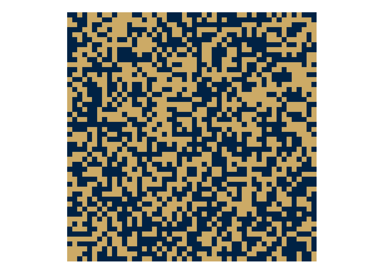
To simulate such a system, we first begin with random states on a lattice. This is our initial \(s\).
We then randomly select a focal state somewhere on the lattice
i =sample.int(N,1)j =sample.int(N,1)
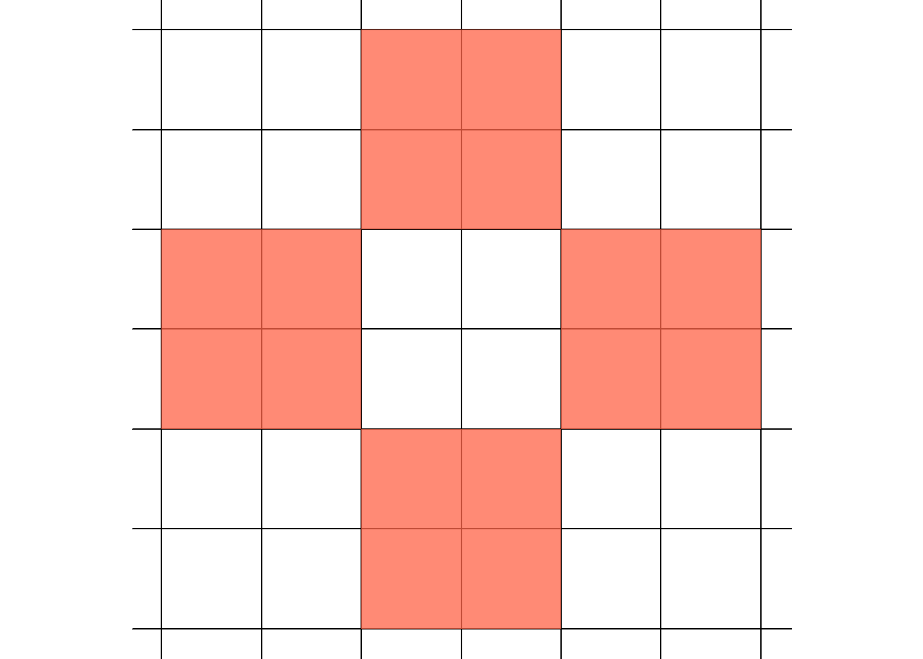
and then identify the neighbors of \(i\) and \(j\). In this case, we identify the von Neumann neighborhood. This is done using some indexing tricks to deal with indexing that begins at 1 instead of 0, and to ensure that the neighborhood wraps around the lattice (no edge effects).
neighbor_sum =function(i,j,S) { up = S[(i-2) %% N+1, j ] down = S[ i %% N+1, j ] left = S[ i, (j-2) %% N+1] right = S[ i, j %% N+1] up + down + left + right}
When combined with \(J\) this gives \(H(s)\), which can then be fed into equation Equation 1 to obtain \(P(s)\).
J =1H = J *neighbor_sum(i,j,S) B =0.7P =1/ (1+exp(-2* B * H))
It is worth noting that the function to compute \(P(s)\) takes the general form \(1 / (1 + e^{x})\), which is a logistic transform, otherwise known as the binary softmax. This is not a defining feature of the model. It arises out of necessity when going from discrete states into probabilities. It is the plumbing, and not the flow.
The flow comes from the local neighborhood configurations \(s_is_j\) combined with \(\beta\) and \(J\).
The final step then is to generate the new state given the probability.
ifelse(runif(1) < P, 1, -1)
[1] 1
Putting this together, we have a function with which we can loop over focal states and then make updates.
ising =function(N, beta =0.7, J =1, n_steps) {# states S =matrix(sample(c(-1,1), N*N, replace = T), N, N)# neighbor sum neighbor_sum =function(i,j,S) { up = S[(i-2) %% N+1, j ] down = S[ i %% N+1, j ] left = S[ i, (j-2) %% N+1] right = S[ i, j %% N+1] up + down + left + right }# loop for(t inseq_len(n_steps)) { i =sample.int(N,1) j =sample.int(N,1) H = J *neighbor_sum(i,j,S) P =1/ (1+exp(-2* beta * H)) S[i,j] =ifelse(runif(1) < P, 1, -1) } S}
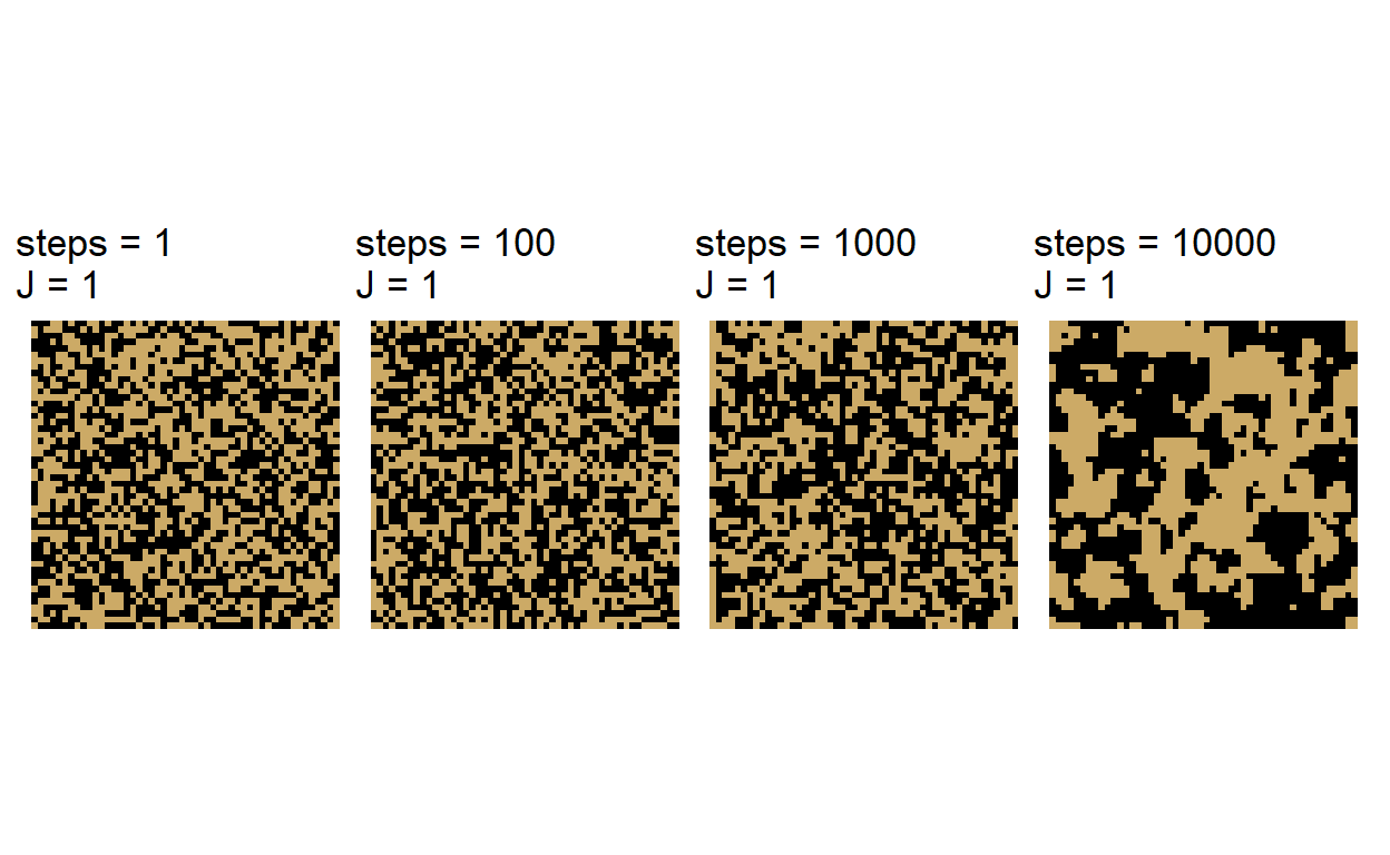
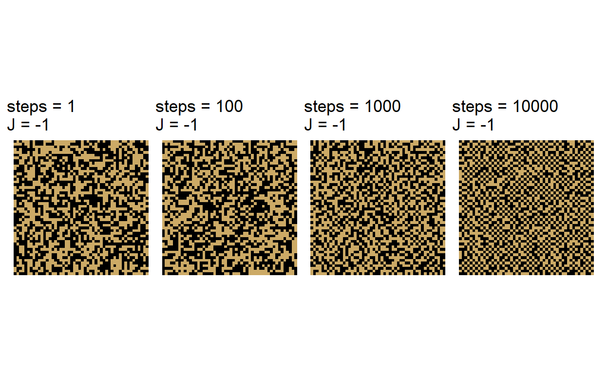
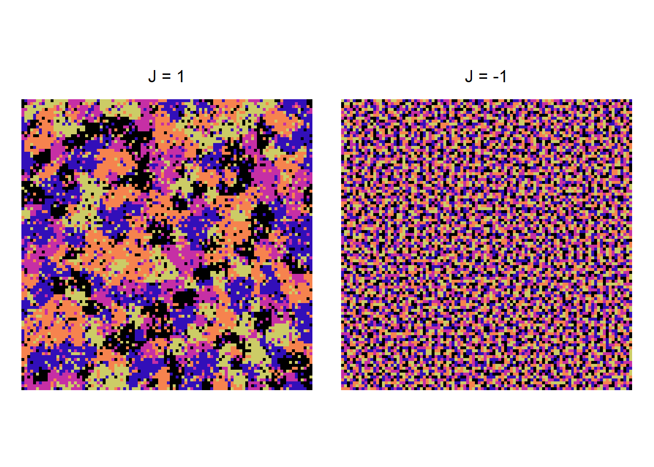
\(J\) has a significant effect on the configuration that emerges over a sequence of updates. When \(J > 0\), we observe a facilitation effect where neighbors of the same state grow into cluster.
One way to extend this simulation is to allow more flexible neighborhoods. We do this by defining offsets, and use these to index the neighbors for a focal state.
make_neighbors =function(offsets, N) {function(i, j) { ii = (i + offsets[,1] -1) %% N +1 jj = (j + offsets[,2] -1) %% N +1cbind(ii, jj) }}
make_neighbors is a function factory that takes in the offsets (a vector of locations around a focal state) and the size of the lattice N, and provides a function that can lookup this neighborhood for a given \(i\) and \(j\) (much like the first portion of neighbor_sum). This makes the simulation much more flexible.
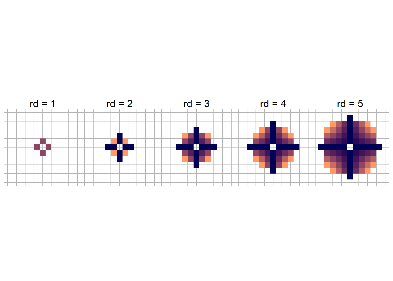
A fun example is to generate disk offsets. Rather than indexing directions by hand, we can define a disk with radius rd. For instance, if rd = 1, then we get the familiar von Neumann neighborhood.
Here we provides functions to make neighbors based on offsets, generate disk offsets, and then update the ising function to include these extensions.
# neighborhood make_neighbors =function(offsets, N) {function(i, j) { ii = (i + offsets[,1] -1) %% N +1 jj = (j + offsets[,2] -1) %% N +1cbind(ii, jj) }}# disk function disk_offsets =function(rd) { disk =as.matrix(expand.grid(-rd:rd, -rd:rd)) disk = disk[rowSums(disk^2) <= rd^2&rowSums(disk^2) >0,]return(disk)}ising =function(N, beta =0.7, J =1, n_steps, offsets) {# states S =matrix(sample(c(-1,1), N*N, replace = T), N, N)# neighborhood function neighbors =make_neighbors(offsets, N)# loop for(t inseq_len(n_steps)) { i =sample.int(N,1) j =sample.int(N,1) n =neighbors(i,j)# hamiltonian and partition H = J *sum(S[n[,1], n[,2]]) P =1/ (1+exp(-2* beta * H)) S[i,j] =ifelse(runif(1) < P, 1, -1) } S}
Potts Example
Now let’s turn to the Potts model. This code looks very simulate to the previous, except that instead of summing across all the states, we use tabulate to retrieve the frequency of the states within the neighborhood. All other changes are to extend the model to q states (e.g., seq_len(q)).
potts =function(N =50, q =5, beta =0.5, J =1, n_steps =1e4, offsets) { S =matrix(sample(seq_len(q), N*N, replace = T), N, N) neighbors =make_neighbors(offsets, N)for(t inseq_len(n_steps)) { i =sample.int(N,1) j =sample.int(N,1) n =neighbors(i,j) neighbor_states = S[n[,1],n[,2]] counts =tabulate(neighbor_states, nbins = q) p =exp(beta * J * counts) p = p /sum(p) S[i,j] =sample(seq_len(q), 1, prob = p) } S}
The Ising and Potts models generate a probability distribution over discrete spatial configurations using energy-based (Gibbs) neighborhood interactions (Wu 1982). Spatial patterns emerge from these local interactions. To simulate these models, we use local stochastic updates which typically converge to a stationary distribution. Spatial configurations exhibit an apparent “criticality” for a give size of the lattice on which the patterns are generated.
Core equations
Both the Ising and Potts models are based on the following equation
where \(s\) is the full configuration, \(\langle i,j \rangle\) are the neighbors, \(J\) is the interaction strength, \(\beta\) is the inverse temperature (the decision sharpness/stochasticity), and \(Z\) is a partition that normalizes the states to probabilities.
For the Ising model, \(s_i \in \{-1,+1\}\) while in the Potts model \(s_i \in \{1,...,q\}\).
In order to update the state of a focal cell at each step, the sum of the neighbor states must be transformed to a probability. For the Ising model, this is a logistic transform or a binary softmax
Here the notation \(\partial_i\) denotes the neighborhood distance (e.g., rd) and all \(j\) who fall into this neighborhood. Such transformations have no definitive influence on the spatial configurations; they merely normalize the probabilities (Newman and Barkema 1999).
Stationarity and Phase Transitions
Because Gibbs updates on a lattice are an example of a Markov chain (Binder, Heermann, and Binder 1992), there is a unique stationary distribution for any finite value of \(\beta\). When \(\beta\) is large or near criticality, mixing is slow, making the stationary distribution difficult to find without extended computation.
Because a true critical point is only defined when \(N \rightarrow \infty\), in a fixed lattice, one can only find a pseudo-critical value \(K^*(N)\) where \(K = \beta J\). At \(K^*\), fluctuations are approximately critical. Importantly, different neighborhoods will change the nature of the interactions and this \(K\) will shift.
At this pseduo-critical point, we observe scale-free spatial patterns and diverging correlation lengths. To find this point, we hold \(N\) contant and then sweep through \(\beta J\). For each \(K\), we sample the equilibrium magnetization values
\[\begin{align}
m_1, ..., m_T
\end{align}\]
and compute fluctation based summaries (means) at \(\langle m^2 \rangle\) and \(\langle m^4 \rangle\). \(K^*\) occurs where the fluctuations are greatest.
References
Binder, Kurt, Dieter W Heermann, and K Binder. 1992. Monte Carlo Simulation in Statistical Physics. Vol. 8. Springer.
Newman, Mark EJ, and Gerard T Barkema. 1999. Monte Carlo Methods in Statistical Physics. Clarendon Press.
Wu, Fa-Yueh. 1982. “The Potts Model.”Reviews of Modern Physics 54 (1): 235.