Primary or Secondary? – Shane A. Scaggs

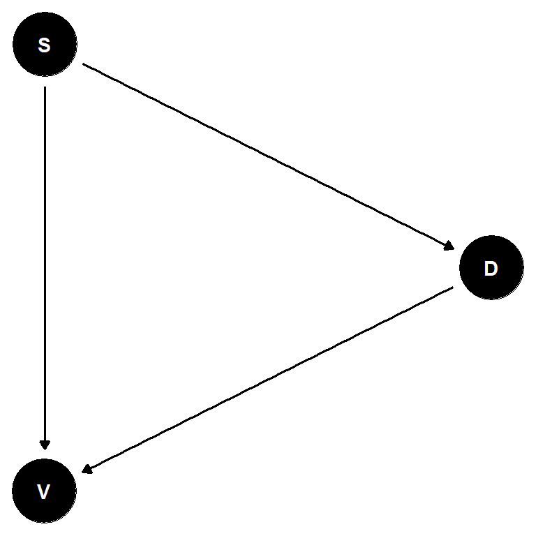
Let’s suppose we are interested in the relationship between disturbance (D) and vegetation diversity (V). We assert that disturbance has a causal effect on diversity such that \(D \rightarrow V\).

Both disturbance and vegetation diversity arise from spatial processes, and the data we use to study them are collected in space. This makes it natural to assume that there may be some spatial autocorrelation in these measures. We might think it is simply a question of how to control for this autocorrelation so that we can get a precise estimate of the effect of D on V. For example, we might use a conditional autoregressive model, treating D and V as emissions from a random field.

However, I argue that rather than assuming we must control for autocorrelation, we need o first determine whether we need to adjust for autocorrelation by looking at the problem from a causal inference perspective.

A Joint Spatial Process

For example, let’s suppose that D and V arise jointly from a spatial process S.

library(dagitty)
library(ggdag)
library(ggplot2)

dag2 = dagify(
  V ~ D, 
  D ~ S, 
  V ~ S,
  exposure = 'D', 
  outcome  = 'V'
)
ggdag(dag2, layout = 'circle') + theme_void()

This DAG says that both of our measures, D and V, are caused by the same spatial process. Put differently, the effect of D on V is confounded by spatial autocorrelation in these variables. This implies that we must include S in a model.

ggdag_adjustment_set(dag2) + theme_void()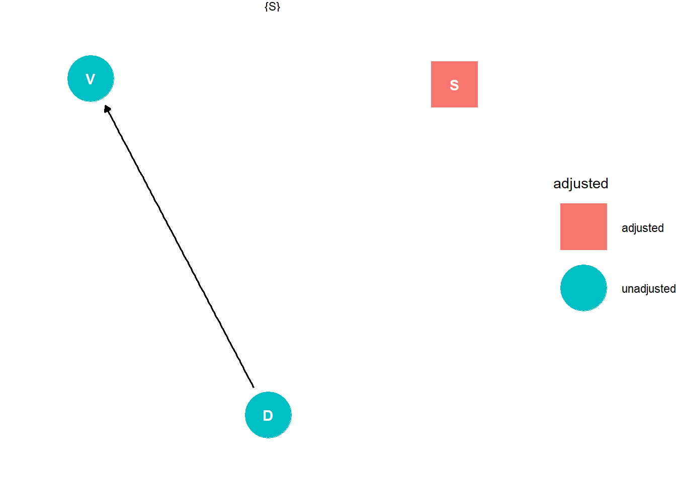

Simple enough. But is this actually plausible? If true, then disturbance and vegetation diversity must both occur at a similar scale. This is a strong assumption considering that measures of vegetation diversity occur at the organism or stand level, whereas disturbance is typically a patch level phenomenon. If there is spatial structure to these measures, they would occur at distinct scales.

Moreover, the processes that underlie this spatial structure are probably distinct. Disturbances, for example, can be due to tree-falls, hurricanes, landslides, anthropogenic land changes, diseases or pest outbreaks, and so on. These are quite different from the processes that shape vegetation diversity like local competition, facilitation, and mutualism; dispersal and recruitment; or nutrient availability.

Independent Spatial Processes

It seems more likely that D and V have their own spatial patterns arises from distinct processes. This implies a DAG like this:

dag3 = dagify(
  V ~ D, 
  D ~ S_D, 
  V ~ S_V,
  exposure = 'D', 
  outcome  = 'V'
)
ggdag(dag3, layout = 'tree') + theme_void()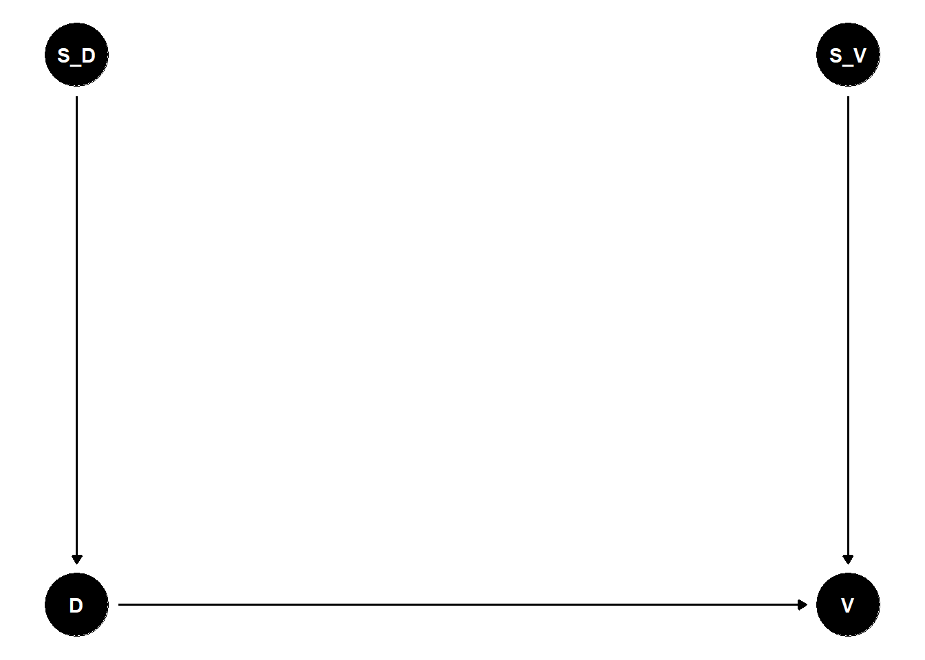

If this is our generating process, then we need to be much more careful about including S_D and S_V in a model.

ggdag_adjustment_set(dag3) + theme_void()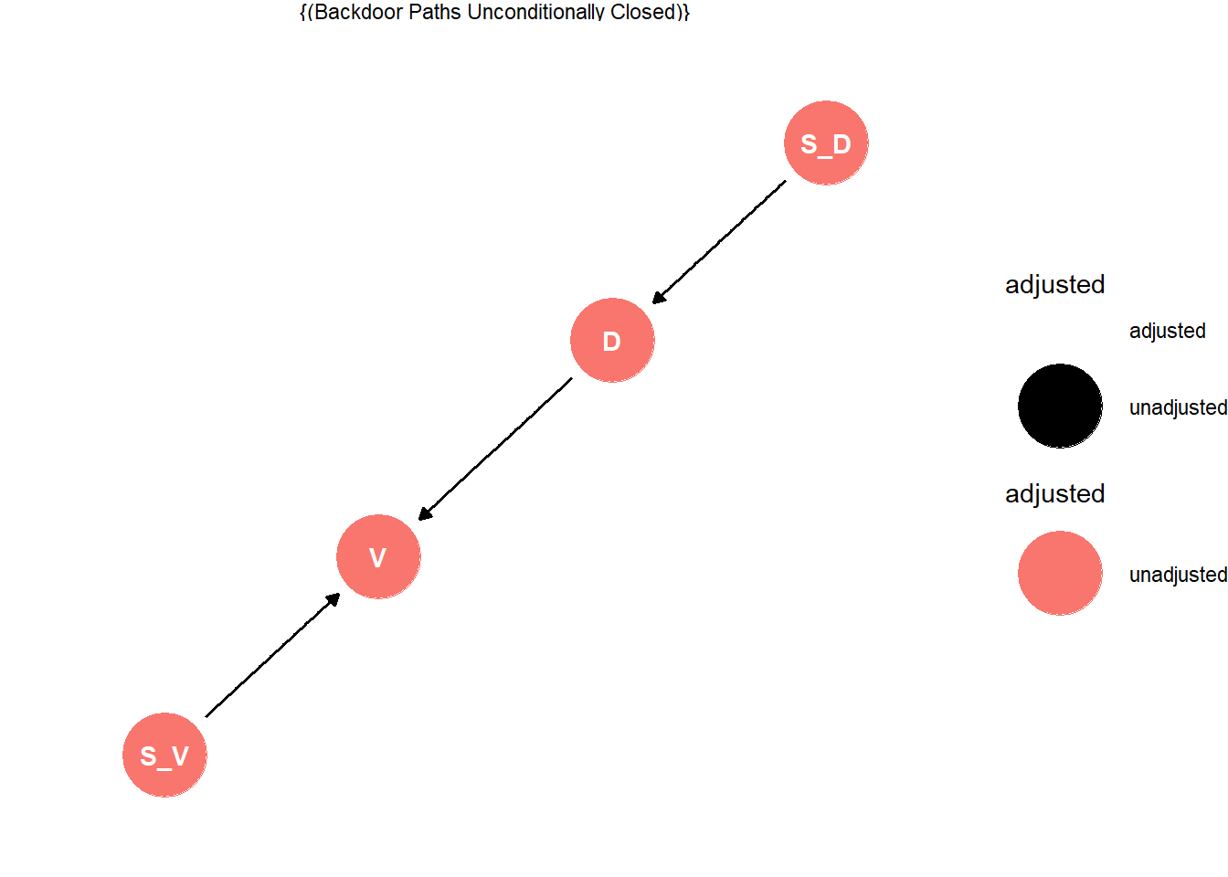

The current structure contains no backdoor paths. If we include S_D, for example, then we will filter our any effect of D that is correlated with S_D. One could then ask: “Why not condition directly on S_D and leave our D, altogether?” This could work but only if we know that the variation in S_D is due solely to the disturbance. S_V does not have these same issues We could include S_V as a covariate that might improve the precision of our estimate of D on V.

Primary and Secondary Structure

Now here is where this gets interesting. S_D and S_V are what some might call “secondary spatial structure”. They are patterns of vegetation and disturbance that are overlaid on the landscape with all its topography and geomorphology – the primary spatial structure. One could very reasonably assume that this primary structure influences the secondary structure. Indeed, many have debated this tension in the literature. A DAG representing this might look like the following:

dag4 = dagify(
  V ~ D, 
  D ~ S_D, 
  V ~ S_V,
  S_D ~ P, 
  S_V ~ P,
  exposure = 'D', 
  outcome  = 'V'
)
ggdag(dag4, layout = 'tree') + theme_void()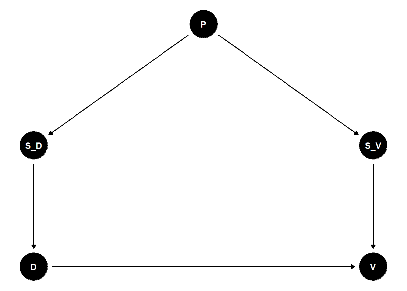

Now we again have a backdoor between D and V through the influence of P on S_D and S_V. This means that in order to estimate the relationship between D and V, we must adust for P, assuming that we have a measure of it.

ggdag_adjustment_set(dag4) + theme_void()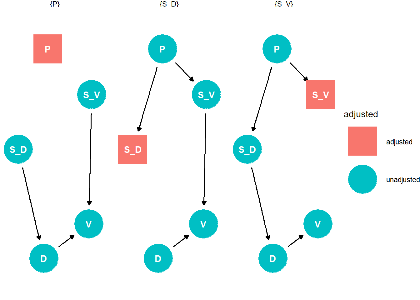

Further, one can break the backdoor path by adjusting for any of the parents of D and V. However, we must be careful here about what we actually mean by P. For all we know, P could represent physical laws. If that is the case, then pretty much any DAG we ever draw would be confounded! What began as a relatively simple modeling problem has taken us to a deeply philosophical place where we question whether we can ever really know the causal effect of anything…

Okay, that was a little unserious. Of course we can know causal effects. And P in the graph cannot be the fundamental laws of physics. Even if they were, they would be constants and so they would do little to shape any variation in these variables.

The more prudent question is whether there is an ultimate common cause of spatial structure.